
Verification or optimisation? The hidden cost of phased-array workflows
From unit-cell analysis to finite arrays: where phased-array workflows can be improved
Phased-array development moves through several distinct analysis stages. A unit-cell model is useful for element design under periodic assumptions. A finite-array model is required when the complete aperture must be analysed. Beamforming synthesis and excitation optimisation introduce further design variables. The efficiency of this workflow influences not only how quickly a design can be evaluated, but also how many design alternatives can realistically be explored before engineering decisions are made.
The methods used at each stage are well established. The practical difficulty lies in the transition between them. Geometry, material definitions, excitation states, scan conditions, and phase references must be transferred or reset at each transition, and where full-wave analysis is expensive, the transition cost also limits how many design alternatives are evaluated.
The relevant question is therefore not only whether a tool can perform an analysis. It is whether the workflow allows engineers to move efficiently between analysis stages and iterate enough to explore the design space before engineering decisions are made
A design can pass verification even when only a small part of the intended design space was explored. That limitation is not visible in the final results, because it lies in the candidates that were never evaluated.
From a periodic model to a finite array
Mutual coupling separates element-level characterisation from finite-array analysis. Each element radiates into an environment created by its neighbours, and that environment depends on array size and layout, lattice spacing, and scan angle. The embedded element pattern is not the isolated element pattern, and the active reflection coefficient is not the standalone S11.
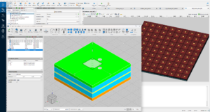 |
A unit-cell model with periodic boundary conditions represents an element surrounded by an infinite periodic lattice. Considering infinite array conditions using Floquet excitations, this gives quantities such as the active reflection coefficient and the embedded element pattern as functions of scan angle, at a cost that allows iteration on the element itself. |
It also does not represent the edges of a finite array, or any aperiodic layout, where elements see a different electromagnetic environment from elements in an infinite lattice. When edge behaviour is relevant to the design, the array must be analysed as a finite structure. The same applies when a radome or another nearby structure affects the array.
Moving between models and representations is costly, and that cost depends heavily on the tools in use. Where the two models are built in separate environments, the element geometry and the frequency definition typically transfer. The following are defined again:
- the finite lattice, the amplitude taper, the edge configuration ,and the scan definitions;
- Excitation amplitude and phase distributions, generated in one environment and applied in another;
- Port numbering, coordinate systems and phase references, which must remain consistent if results from the two models are to be compared.
This procedure is repeated each time the element geometry changes. Each task is small on its own, but what matters is the cumulative cost over many design iterations and this transfer work is the part of the loop that does not benefit from a faster machine.
Manual transitions also introduce inconsistency between models: a phase convention applied differently, or an excitation distribution normalised in another way. The resulting discrepancy is difficult to distinguish from genuine electromagnetic effect. When the transition is cheap, engineers check finite-array behaviour while the element design can still change. When it is expensive, that check tends to be postponed until the element design is effectively fixed.
Full-wave analysis limits the practical design space
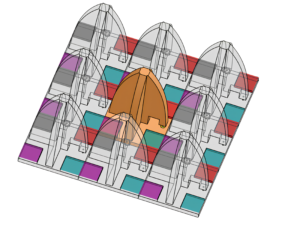
There is a difference between being able to analyse a finite array and being able to iterate on it. Full-wave analysis becomes more demanding as array size and model complexity increase: detailed feeds, multilayer structures, and fine geometric features increase both computation time and memory use. A study across a scan volume or a frequency band requires many solutions rather than one.
| A memory limit is more restrictive than a time limit, because a model that exceeds the available resources cannot be analysed at all without changing the model or the method. Engineers then simplify the feed, reduce geometric detail, analyse a smaller subarray or use another approximation. Each choice can be technically justified. The important point is whether the choice is based on the analysis required or on the available computational resources. | 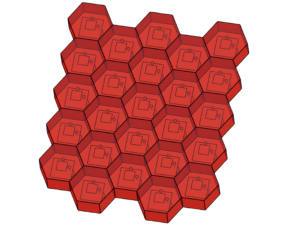 |
 |
Consider an illustrative design study in which several element and lattice configurations must be compared before a design review. If each full-wave analysis has a long turnaround time, the number of configurations evaluated is determined by the calendar rather than by the remaining engineering questions. A configuration may then be excluded because it was never analysed, not because it performed poorly. |
This is the distinction between verification and optimisation. Verification establishes that a selected design meets its requirements; optimisation establishes whether a better design exists within the relevant design space. A design can pass verification even when only a small part of the intended design space was explored. That limitation is not visible in the final results, because it lies in the candidates that were never evaluated.
When the engineer becomes the optimisation loop
Beamforming synthesis, complex excitation coefficients, and element spacing are design variables. Where they are treated as checks applied after analysis, the loop connecting them is manual:
- adjust the design or excitation parameters;
- Update or transfer the model;
- Run the analysis;
- Review pattern, impedance and coupling results;
- Select the next change, and repeat.
This has three consequences.
The number of candidates evaluated is set by how many cycles fit into the available time, so iteration is limited by the engineer’s time as well as by computational resources. Interactions between variables are harder to study: when element spacing, excitation taper and edge configuration affect the same result, changing one parameter at a time may not reveal the best combination. Finally, model updates, transfers, and consistency checks consume specialist engineering time.
Integrated optimisation does not replace engineering judgement. It allows that judgement to be applied to more candidates and parameter combinations than a manual process normally supports, and it keeps synthesis and full-wave validation connected.
Questions to test the workflow
These questions apply to any phased-array design process, including one assembled from tools you may already own.
- Can the design move from periodic analysis to finite-array full-wave analysis without rebuilding the model, and which definitions must be recreated or transferred manually?
- Do computation time and memory use scale predictably to the largest required array, or do resource constraints determine the analysis method?
- Can enough candidates be evaluated to support optimisation, or only enough to verify a selected design?
- Are beamforming synthesis and excitation optimisation connected to the analysis environment, and can array-level feedback be obtained before committing to a full-wave analysis?
- How many exports, imports, and manual consistency checks are required during one optimisation cycle?
If the answers involve repeated rebuilding, waiting or manual checking, the limitation may not be one individual solver. It may be the cost of moving between analysis stages.
What improved workflows cannot solve
Not every phased-array challenge is caused by workflow. Wideband element design, scan blindness, feed network loss, manufacturing tolerances and calibration remain difficult engineering problems, and full-wave analysis of a large finite array remains computationally expensive even with an efficient solver. Nor is every handoff a problem, since scripted and well-tested interfaces can make transitions efficient. In some cases the right approach is to reduce the design space or accept additional margin rather than perform more iterations.
A better workflow does not remove the underlying electromagnetic or computational challenges. It reduces the additional work required to move between the methods used to address them.
How ARRAY supports this workflow
ARRAY was designed to reduce the cost of moving between the main stages of phased-array analysis and optimisation by bringing them together in one environment.
Elements can be analysed as standalone elements or under infinite-array assumptions, and the same model definitions are used for full-wave analysis of the finite array rather than being defined again in a separate environment. Array Liveplot provides analytical array-level feedback during synthesis before a full-wave analysis is started. The Fast Direct Solver is designed to make the analysis of large finite arrays more tractable in computation time and memory. Beamforming synthesis and excitation optimisation are integrated into the design environment, reducing the need to assemble the iteration loop through manual exports and imports.
 If you are ready to optimise your operations and drive faster outcomes, read more about ARRAY through the Solution Sheet.
A 60-day trial licence is available for teams that want to evaluate ARRAY using their own array designs, with access to TICRA engineers throughout the evaluation.