Random surface distortion in GRASP
Surfaces with random distortions are encountered in many practical antenna problems, e.g., when a reflector antenna is manufactured to a specific surface tolerance or it is subjected to wear and tear during its lifetime. As increasingly higher frequencies are used in reflector systems, it becomes more and more important for the antenna engineer to be able to accurately estimate the effects of surface distortions.
In this white paper, we describe how the scattered field from a surface with random distortions can be calculated by GRASP and how these results correspond to the widely used Ruze equations.
Download as PDF
Random surface error model
Random surface errors in GRASP are defined by the two values ns and εp. The random surface is generated by covering the reflector by a regular grid with a node spacing ns along both axes of the grid. The surface offset at the nodes of the grid is selected as random numbers uniformly distributed in an interval with the peak-to-peak value 2εp and a mean value of zero. A cubic interpolation function connects the grid points and yields a continuous surface between the random values at the nodes. This means that within a square with side lengths 2ns the surface distortions are correlated, whereas they are nearly uncorrelated for larger distances.
It can be shown that the cubic interpolation used in the GRASP random surface leads to an rms value, εrms, equal to the selected peak value, εp, times a correction value stemming from the cubic interpolation of 0.47, i.e., εrms = 0.47 · εp
The spacing between the nodes, ns, determines the smoothness of the surface. A larger value of ns results in a slower variation across the surface, and thus a smoother surface. On the other hand, smaller values of ns provide a more rapidly varying surface.
Five cases of surface smoothness corresponding to ns = 1.2, 0.6, 0.24, 0.12, and 0.06 mm for the same value of εrms are illustrated in Figure 1.
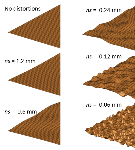
Figure 1 -The surface for different smoothness. The distance between the black lines on the surface is 0.06 mm. Only a corner of the plate is shown.
Correlation length
A common source of confusion when dealing with rough surfaces is the different definitions of correlation length used in different professions. In his examinations of reflector antennas, Ruze based his equations on a concept of a correlation region with diameter “2c” outside of which the correlation is zero. Another more general definition of the correlation length Lc, which is widely used in optics, is the distance from the peak of the autocorrelation function, ACF, at which the ACF has dropped to a value e -1 below the peak.
To illustrate the two different definitions and how they relate to the node spacing ns used in GRASP, a rough surface with a grid spacing of ns = 5 mm and εp = 0.5 mm is shown in Figure 2. The autocorrelation function, ACF, of this rough surface is shown in Figure 3.
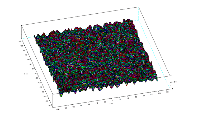
Figure 2 – The surface shape for 5 mm grid. Unit in mm.
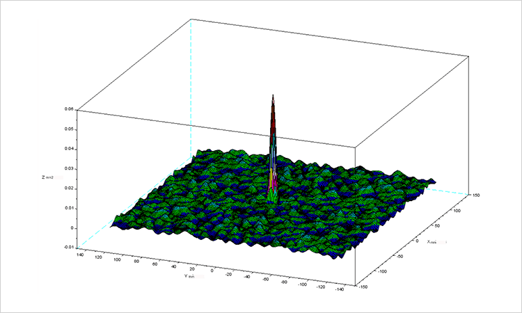
Figure 3 – Autocorrelation function for surface in Figure 2.
The autocorrelation function in the cuts through the peak along x and y are shown in Figure 4 and Figure 5, respectively.
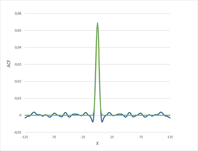
Figure 4 – Autocorrelation function for Y=0 and the Gaussian approximation with σ = 2.5 mm.
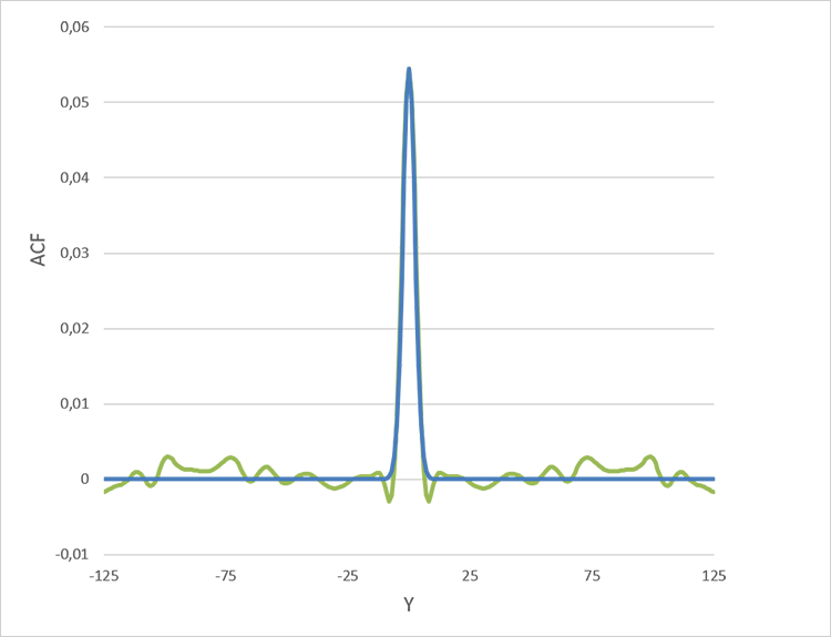
Figure 5 – Autocorrelation function for x=0 and the Gaussian approximation with σ = 2.5 mm.
The peak value of the autocorrelation function, ACF(0) = 0.0544519, corresponds to an rms surface error, εrms = √ ACF (0) = 0.2333494mm ≈ 0.47εp, which is in good agreement with the expression in (1).
The correlation length Lc , defined as the distance at which the value of the autocorrelation function is e -1 of the peak value, is Lc = 3.86 mm ≈ 0.77 ns.
It is seen that the distance between the first two minima of the autocorrelation function is approximately 10 mm, or 2c, thus corresponding well to Ruze’s definition of correlation distance. In other words, it is sensible to compare the results of Ruze for a correlation region of 2c to those of GRASP with a node spacing of ns.
Ruze equation for RF performance
Random errors on a reflector surface will scatter the field from the forward direction into the side lobe region thereby reducing the peak gain and increasing the side lobes. The standard Ruze formula, which is derived for a plane wave incident on a planar surface with a random distortion with 2c ≥ λ, states that the peak gain is reduced by the factor

For a reflector antenna the equation must be changed to:
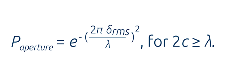
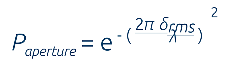
where δrms is the root mean square aperture error in metric units and 2π δrms /λ is the rms aperture field phase error, see Figure 6. Notice, that this gain reduction is in the boresight direction, normally θ = 0°.
For a simple offset reflector as in Figure 6 the aperture error is found by: δrms = (1 + cos (ν )) · εrms
The disturbance of the RF field outside the main beam is also estimated by Ruze, where the average level ofthe distortion field in the sidelobe region is given by
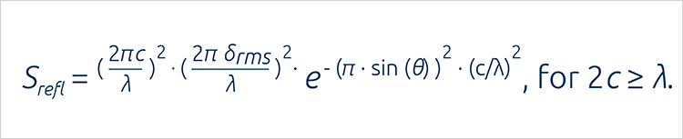
where θ is the angle measured from the boresight direction.
The relation is illustrated graphically in Figure 7 for δrms = 0.02λ. Note that the distortion pattern is independent of the reflector size. The expression is not valid near the axis, θ = 0°, where instead equation (3) should be used.
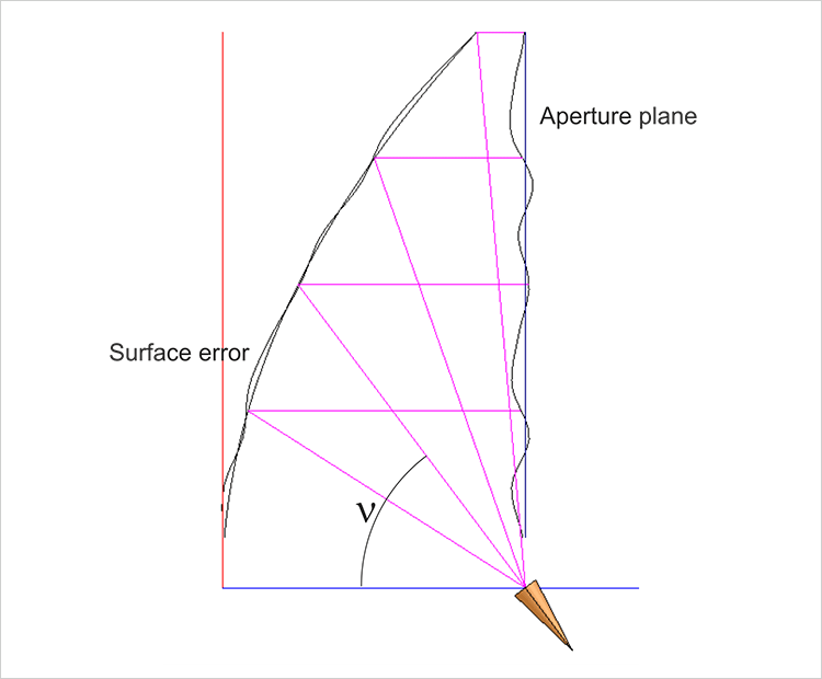
Figure 6 – Aperture error for offset reflector.
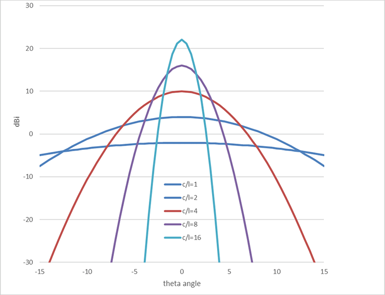
Figure 7 – Ruze distortion field for random surface error with δrms = 0.02λ.
Gain-Loss comparisons
In this chapter the gain loss is calculated by both Physical Optics (PO), which is available in GRASP, and the Method of Moments (MoM), which is available in ESTEAM, and compared with those predicted by the Ruze equations above. The analysed reflector is a plane PEC plate at the frequency of 500 GHz corresponding to a wavelength λ = 0.6 mm. The side length of the square PEC plate is 12 mm (20λ).
First, the plate is illuminated by a plane wave, which is the assumption for the Ruze equation, and secondly,by a tapered Gaussian beam.
Plane-Wave Illumination
The plate is illuminated by a plane wave orthogonally from the front as illustrated in Figure 8.
For reference, the reflected far field from the plate with no surface distortions is calculated by both Method of Moments (MoM) and Physical Optics (PO). The result is shown in the first line in Table 1. Both MoM and PO give a directivity of 38.06 dBi and the patterns obtained with MoM and PO are identical.
Peak loss as function of aperture error
Random errors on the reflector surface will scatter the field from the forward direction into the side lobe region thus reducing the peak gain and increasing the side lobes. The standard Ruze formula (2) states that the peak gain in the boresight direction is reduced by the factor
where it is assumed that 2c ≥ λ. The limitation of this equation regarding the size of the surface error εrms is investigated first. A value of c = 1.2 mm and thus 2c = 4λ is selected and the surface roughness corresponding to the aperture errors of δrms = 0.063 λ to 0.251 λ is used in the calculations.
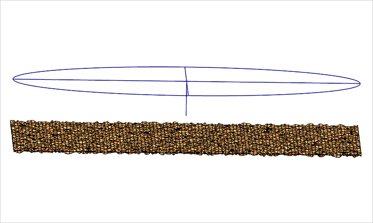
Figure 8 – Distorted plate and plane-wave illumination.
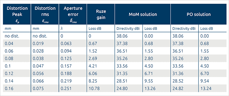
Table 1 – Peak directivity of the scattered beam as a function of the distortion peak. Node spacing ns = 1.2 mm = 2λ.
The scattered field is calculated by both MoM and PO and the resulting peak directivities are shown in columns 5 and 7 of Table 1 for the MoM and the PO solutions, respectively. The loss relative to the non distorted surface is presented in columns 6 and 8. The gain losses as predicted by the Ruze equation in column 4 show that for a distortion larger than an aperture error of δrms = 0.1λ the estimates by Ruze are too low. This is due to the arising 2nd order effects in the basic Ruze equation. The agreement between MoM and PO is very good for all aperture errors, see Figure 9.
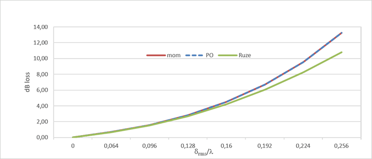
Figure 9 – Peak loss as function of aperture error. Point distance c 0 1.2 mm = 2λ.
We conclude that if the aperture error δrms > 0.1λ, Ruze’s equation for gain loss is inaccurate.
Loss as function of node spacing ns
In the following we will investigate five cases of different node spacings ns = 1.2, 0.6, 0.24, 0.12, and 0.06 mm as shown in column 1 of Table 2. A peak value of εp = 0.04 mm giving a δrms = 0.032 mm and a gain loss of 0.7 dB according to Ruze is selected. The resulting surface shapes are illustrated in Figure 1.
It is clear that the assumption of a correlation distance larger than the wavelength, 0.6 mm, is not fulfilled for all correlation distances, as shown in column 2 of Table 2, and we can therefore not expect the Ruze formula to be valid for these correlation distances.
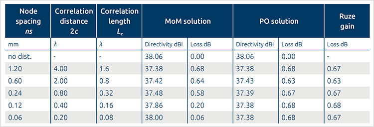
Table 2 – Peak directivity and loss of scattered beam as a function of the node spacing ns. Surface roughness εrms = 0.032 λ.
The scattered field is calculated by MoM and PO and the resulting peak directivities are shown in columns 4 and 6 of Table 2 for the MoM and the PO solutions, respectively. The loss relative to the non distorted surface is presented in columns 5 and 7. The results show that for node spacings of ns = 1.2 mm and 0.6 mm, where the diameter of the correlation region as defined by Ruze is larger than the wavelength, the agreement between MoM and PO is very good and the directivity loss is well predicted by Ruze. The difference in the results for ns = 1.2 mm and 0.6 mm is caused by the change of the number of sample points in the random surface distortion. To simulate a smaller correlation length, the number of random points must be increased.
Decreasing the node spacing to ns = 0.24, 0.12, and 0.06 mm leads to deviating results in the MoM and PO solutions, and for the most rough surface, c = 0.06 mm, the PO solution deviates significantly from the more correct MoM result as can be seen in Figure 10.
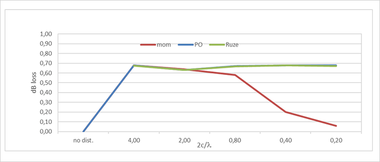
Figure 10 – Peak loss as function of the correlation distance used by Ruze. Aperture error δrms = 0.064 mm.
Another observation is that when the correlation distance becomes less than a wavelength, the loss in peak gain as predicted by the MoM analysis decreases and for ns = 0.06 mm it is only 0.06 dB. This behaviour can be explained by the following considerations.
If a plane wave illuminates a plane surface with periodic distortions with a period less than a wavelength, all the incident power will be reflected in the specular direction independent of the amplitude of the distortion. Imagine now that we make a Fourier expansion of the surface in Figure 8 for ns = 0.06 mm. This expansion will contain a number of harmonics with a period smaller than the wavelength which will therefore not contribute to the directivity loss. Only the harmonics with a period larger than the wavelength will contribute, and they will play a smaller role the faster the surface variations are. Therefore, the directivity loss decreases with decreasing c.
We conclude from the above that for 2c < λ , both PO and the Ruze gain loss equation give too large values and MoM must be used to calculate the radiation pattern.
Tapered illumination
The influence of a tapered illumination, more similar to the feeds used in real-life reflector antennas, is investigated in this section. The flat plate from above is now illuminated by a Gaussian beam with six different waist sizes, w0, in the interval from 1 mm to 6 mm. The waists are located on the plate surface as illustrated in Figure 11.
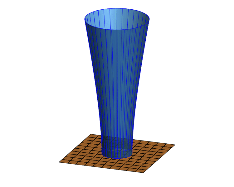
Figure 11 – Random distorted plate illuminated by a Gaussian beam. The waist is located at the nominal surface of the plate.
This generates a tapered field on the plate with a constant phase, see Figure 12.
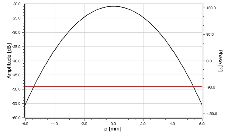
Figure 12 – Field strength (black) and phase (red) of Gaussian beam at the surface of the plate. Waist size w0 = 3mm.
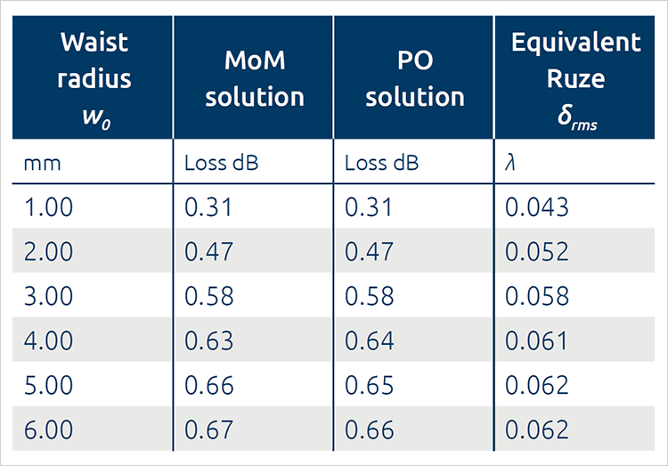
Table 3 – Gain loss of the scattered beam as a function of tapered illumination, c=1.2 mm.
The random surface is created using εp = 0.04 mm and a node spacing ns = 1.2 mm. The assumption of a Ruze correlation region with a diameter greater than the wavelength of 0.6 mm is fulfilled, and we would therefore expect the Ruze gain-loss equation to be valid. and the PO and MoM gain calculations to be identically, which is shown in Table 3 and Figure 13.
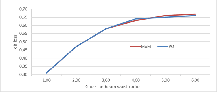
Figure 13 – Loss in peak calculated with PO and MoM as function waist radius w0. Node spacing ns = 1.2 mm.
In Table 2 it was shown that Ruze’s formulation, which does not account for the taper, would predict a loss of 0.67 dB for this case. We can derive an “equivalent” Ruze aperture rms error that would lead to the same gain loss as predicted by PO, and this is shown in column 4 of Table 3.
It is evident that the aperture rms error, δrms, in the Ruze equation of the gain losses must be corrected with the weights given by a tapered illuminated field. The equivalent weighted and the unweighted aperture rms errors, δrms, as a function of the Gaussian beam waists are shown in Figure 14.
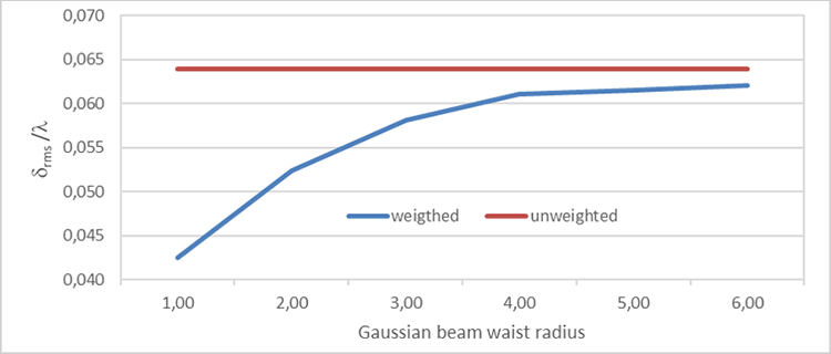
Figure 14 – Equivalent aperture error.
When the Gaussian beam waist increases giving a constant illumination of the plate, the weighted aperture error is approaching the total rms value. The influence of the node spacing is considered by looking at the losses for five different node spacings, ns = 1.2, 0.6, 0.24, 0.12, and 0.06 mm using a tapered illumination. In order to get a low illumination at the plate edges and still have a reasonable plate size a beam waist radius of 1 mm is selected.
First, we investigate the case where the plate has no surface distortions. The reflected peak gain from the plate calculated by both Method of Moments (MoM) and Physical Optics (PO) is shown in the first line in Table 4. Both the MoM and the PO solution give a directivity of 23.45 dBi.
The same random errors as for the previous plane wave illumination with a peak value of 0.04 mm are used in this case. The resulting peak directivities are shown in columns 3 and 5 of Table 4 for the MoM and the PO solutions, respectively. The loss relative to the non distorted surface is presented in columns 4 and 6.
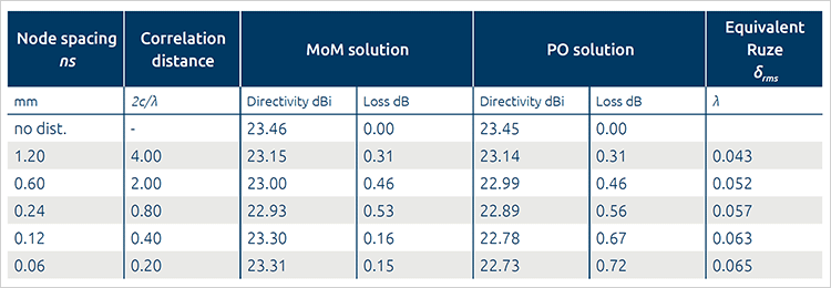
Table 4 – Peak directivity of the scattered beam as a function of the node spacing, δrms = 0.064 λ.
As for the plane wave illumination the RF results show that for the node spacings ns = 1.2 mm and 0.6 mm, where the diameter of Ruze’s correlation region 2c is larger than the wavelength, the agreement between MoM and PO is very good. Changing towards a more rapidly varying surface distortion by decreasing the node spacing, specifically ns = 0.24, 0.12, and 0.06 mm, the MoM and PO solutions start to deviate and for the most rapidly varying surface distortions, ns = 0.06 mm, the convergence of the PO solution is simply not possible, see Figure 15. Furthermore, as in the plane wave illumination case, the peak directivity of the MoM result starts to increase when the correlation distance becomes less than a wavelength, and for ns = 0.06 mm the loss relative to the smooth surface is only 0.05 dB.
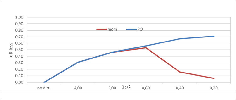
Figure 15 – Peak loss as a function of the surface roughness, δrms = 0.064 mm.
From the losses in the PO calculation an equivalent value of the aperture rms error, δrms, can be found using the Ruze equation. Notice, that the large taper of the Gaussian beam introduces a weight in the rms function of the surface roughness giving different rms values for different correlation lengths The value in column 6 correspond very well to the rms error inside a surface region of 1.2*w0.
We conclude that Ruze’s formula must be corrected for realistic tapered illuminations, which can be done by applying a weighting, similar to the tapering, to the rms value of the distortions. The MoM should be used over PO for 2c < 0.8λ.
For the random surface model in GRASP, defined by the node spacing ns and the peak value εp, the relations to the right holds true. If the aperture error δrms > 0.1λ, Ruze’s equation for gain loss is inaccurate.
If the diameter of the correlation region 2c < λ, both PO and the Ruze gain loss equation give too large values for plane-wave illumination and MoM must be used to calculate the radiation pattern.
Ruze’s formula must be corrected using a weighted rms value for the distortion for realistic tapered illuminations, while PO can be used for 2c > 0.8λ. For smaller values the MoM should be applied.
> More about GRASP
> Download as PDF